General Rhomb Tiling Model.

( Section II of rhomb tiling paper )

We will denote a rhomb prototile with opening angle $s\pi{}/n$ as $T_s^n$ and the corresponding substitution rhomb tile as $S_s^n$ . The model is based on the observation that the combined area of the pair of rhomb prototiles $T_{s+t}^n$ and $T_{s-t}^n$ is proportional to the area of the rhomb prototile $T_s^n$ , the proportionality factor $c_t=2\cos(t\pi/n)$ being independent of $s$ . Consequently, substitution tiles $S_s^n$ may be constructed from a combination of prototiles $T_s^n$ and pairs of tiles $T_{s\pm t}^n$ . If $n_0$ and $n_t$ are their numbers respectively, the ratio of the area of $S_s^n$ and $T_s^n$ is

(1) $\begin{equation*}S=n_0+\Sigma_t 2n_tc_t\end{equation*}$

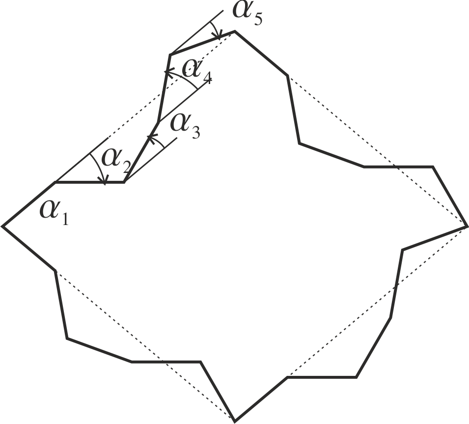
SubstitutionEdgeConfiguration — Fig. M1. Substitution tile edge structure. The edge angles $\alpha_i$ occur in $\pm$ pairs or are zero. In this example we chose the edge angles $\alpha_i$ to be $0$ , $-2\pi/9$ , $\pi/9$ , $2\pi/9$ , $-\pi/9$ respectively. All edges have congruent shapes. The lower and upper left edges are related by a rotation over the opening angle $s\pi/9$ with respect to the left corner. Similarly, the lower and upper right edges are related by a rotation over the opening angle with respect to the right corner. Opposite edges are related by a translation.

A second requirement for a tiling of the entire plane is to realize proper edge substitutions. We will assume that all four substitution tile edges have the same shape. Neighbouring edges at the opening angle are related by a rotation over that angle and opposite edges are related by a translation (Fig. M1). This edge arrangement also ensures that the substitution tile area is equal to the inflated rhomb area, and, therefore, $S$ is equal to the areal scaling factor. The angles between the outer prototile edges and the substitution tile rhomb edge will be called the edge angles $\alpha_i$ . For now, we will assume that overhangs are not allowed and $|\alpha_i|\leq \pi{}/2$ . The length of the substitution tile rhomb edge

(2) $\begin{equation*}L=\Sigma_i\cos\alpha_i\end{equation*}$

is the inflation factor of the rhomb tiles. Because the areal scaling factor $S$ is the square of $L$ , equations 1 and 2 can be combined into

(3) $\begin{equation*}S=\frac{1}{2}\Sigma_i\Sigma_j\{\cos(\alpha_i+\alpha_j)+\cos(\alpha_i-\alpha_j )\}\end{equation*}$

This equality can only be satisfied if the arguments $\alpha_i+\alpha_j$ and $\alpha_i-\alpha_j$ are both equal to an integer times $\pi/n$ for all $i$ and $j$ . There are two solutions: either all angles $\alpha_i$ are equal to an integer times $\pi/n$ , or all of them are equal to a half-integer times $\pi/n$ .

Because the beginning and end of the substitution edge have to be at the endpoints of the substitution tile rhomb edge, the following relationship between the edge angles $\alpha_i$ should be met:

(4) $\begin{equation*}\Sigma_i \sin\alpha_i=0\end{equation*}$

A general solution of is that the edge angles $\alpha_i$ occur in $\pm$ -pairs or are zero.

There are also special solutions. For instance, if one requires that the sum of three terms is zero, one finds that $\alpha_1+\alpha_2=\pi{}/3$ and $\alpha_1+\alpha_3=-\pi{}/3$ . This solution is valid if $n$ is a multiple of 3. An example satisfying this condition is the Lord tiling, having edge angles $\alpha_1=\alpha_2=\pi{}/6$ and $\alpha_3=-\pi{}/2$ \cite{HarrissFrett}. $n=3$ in this case, and the edge sequence is $(\frac{1}{2},-\frac{3}{2},\frac{1}{2})$ . In this paper, however, we will only consider the more general $\pm$ pairing condition.

In the general case equation 3 becomes

(5) $\begin{equation*}n_0+2\Sigma_t n_t c_t =\big(m_0+2\Sigma_r m_r c_r\big)^2\end{equation*}$

(6) $\begin{equation*}n_0+2\Sigma_t n_tc_t=\big(2\Sigma_r m_{r+\frac{1}{2}}c_{r+\frac{1}{2}}\big)^2\end{equation*}$

Equations 5 or 6 determine the type and number of prototiles $T_{s\pm t}^n$ from which the substitution tile can be constructed, once the shape of the substitution tile edge has been chosen. In view of the above considerations, this edge shape may be characterized by a sequence of integers or half-integers, the \textit{edge sequence} $(k_i)_1^N$ , defined by $\alpha_i=k_i\pi{}/n$ , $-n/2\leq k_i\leq n/2$ \cite{Maloney14}.

If the finite edge angles are present as pairs in accordance with equation 4, always a valid solution for the substitution tile is obtained, because both sides may be written as a sum of cosine terms having even valued coefficients. The pairing of the edge angles, therefore, guarantees that the substitution tiles are composed of an integer number of prototiles.

GeneralScheme — Fig. M2. General substitution scheme for a substitution tile $S_s^n$ with a given edge shape. The prototile at position $i$ , $j$ is $T_{s+k_i-k_j}$ , where 4 $k_i\pi/n$ and $k_j \pi/n$ are the edge angles at the upper and lower left edges respectively.

Equations 5 or 6 constitute a connection between the prototile edge angle pairs $m_k$ and the numbers of prototiles in a substitution tile $n_t$ , not their arrangement. The relations do not guarantee that a consistent set of substitution tiles can be found. However, in the following we will show that a general set of substitution rhomb tiles can be constructed for arbitrary $n$ and for an arbitrary substitution tile edge shape.

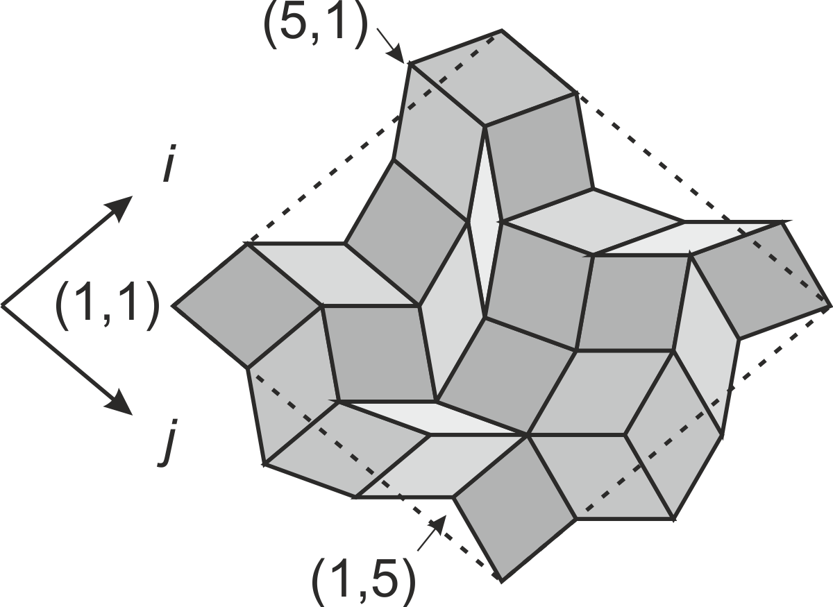
We start with a construction of the circumference of the tile $S_s^n$ as described earlier and illustrated in Fig.~??. Next, copies of the edges are translated to the breaks of neighbouring edges. If the breaks of the upper and lower left edge are indexed as $i\in(1, 2.., n)$ and $j\in(1, 2.., n)$ respectively, starting at the left corner as indicated in Fig.~??), one obtains a grid of vertices $(i, j)$ , at which four prototiles meet. The one bounded by the vertices $(i, j)$ , $(i+1, j)$ , $(i, j+1)$ and $(i+1, j+1)$ is a prototile of the type $T_{s+k_i-k_j}^n$ . The vertices at diagonal positions are occupied by tiles $T_s^n$ , whereas one can find pairs of tiles $T_{s\pm(k_i-k_j )}^n$ at off-diagonal positions $(i,j)$ and $(j,i)$ . This general substitution rule may be represented by the following matrix

(7) $\begin{equation*}S_s^n=\begin{bmatrix}T_s^n &T_{s+k_1-k_0}^n & T_{s+k_2-k_0}^n & \ldots &T_{s+k_{n-1}-k_0}^n \\T_{s+k_0-k_1}^n &T_s^n & T_{s+k_2-k_1}^n & \ldots & T_{s+k_{n-1}-k_1}^n \\T_{s+k_0-k_2}^n &T_{s+k_1-k_2}^n & T_s^n & \ldots & T_{s+k_{n-1}-k_2}^n \\\vdots & \vdots & \vdots & \ddots & \vdots \\T_{s+k_0-k_{n-1}}^n &T_{s+k_1-k_{n-1}}^n &T_{s+k_2-k_{n-1}}^n & \ldots & T_s^n \\\end{bmatrix}\end{equation*}$

For later use one should note, that the prototiles parallel to the substitution edges, i.e. the rows or columns of the matrix, form worms, and the edges of the worms have shapes identical to the edge shape of the substitution tile.

The prototiles are allowed to have indices $s\pm t<0$ or $>n$ . These prototiles will have negative areas, meaning that they have to be subtracted from the tiling. We consider a tiling of the plane to be a legitimate one, if in the end there are no holes or overlaps. So, negative or subtraction tiles are allowed, if they remove all overlaps between tiles and do not leave holes in the tiling. In one of the next sections, we will reason, that this is presumably the case for substitution edges without loops. Also the zero area prototiles for which $s\pm t=0$ or $n$ play a important role in our scheme and cannot simply be neglected.

Substitution Matrices.

Here we want to reformulate the rhomb substitution model in terms of the edge and tile substitution matrices.
If overhangs are included, the prototile edges in a tiling will point into $2n$ directions. Each of these is replaced by a number of prototile edges in orientations determined by the edge sequence, i.e. $m_0$ in the same, $m_n$ in the opposite direction and $m_k$ with $k\in (1, 2,.., n-1)$ in directions differing by $+k\pi{}/n$ and $-k\pi{}/n$ . The edge substitution matrix, therefore, is

(8) $\begin{equation*} \textbf{M}= \begin{bmatrix} m_0 & m_1 & m_2 & \ldots & m_{n-1} & m_n & \ldots & m_3 & m_2 & m_1 \\ m_1 & m_0 & m_1 & \ldots & m_{n-2} & m_{n-1} & \ldots &m_4 & m_3 & m_2 \\ m_2 & m_1 & m_0 & \ldots & m_{n-3} & m_{n-2} & \ldots &m_5 & m_4 & m_3 \\ \vdots & \vdots & \vdots & \ddots & \vdots & \vdots & \ddots & \vdots & \vdots & \vdots \\ m_{n-1} & m_{n-2} & m_{n-3} & \ldots &m_0 & m_1 & \ldots & m_{n-2} & m_{n-1} & m_n \\ m_n & m_{n-1} & m_{n-2}& \ldots & m_1 & m_0 & \ldots & m_{n-3} & m_{n-2} & m_{n-1} \\ \vdots & \vdots & \vdots & \ddots & \vdots & \vdots & \ddots & \vdots & \vdots & \vdots \\ m_3 & m_4 & m_5 & \ldots & m_{n-2} & m_{n-3} & \ldots& m_0 & m_1 & m_2 \\ m_2 & m_3 & m_4 & \ldots & m_{n-1} & m_{n-2} & \ldots & m_1 & m_0 & m_1 \\ m_1 & m_2 & m_3 & \ldots & m_n & m_{n-1} & \ldots & m_2 & m_1 & m_0 \\ \end{bmatrix} \end{equation*}$

A tile with index $s$ is substituted by $n_0$ prototiles with index $s$ , $n_n$ with index $s+n$ and $n_t$ with index $s+t$ and $s-t$ , with $t \in (1,...,n-1)$ and $s \in(0,...,2n-1)$ . So the substitution matrix $\textbf{S}$ is

(9) $\begin{equation*} \textbf{S}= \begin{bmatrix} n_0 & n_1 & n_2 & \ldots & n_{n-1} & n_n & \ldots & n_3 & n_2 & n_1 \\ n_1 & n_0 & n_1 & \ldots & n_{n-2} & n_{n-1} & \ldots &n_4 & n_3 & n_2 \\ n_2 & n_1 & n_0 & \ldots & n_{n-3} & n_{n-2} & \ldots &n_5 & n_4 & n_3 \\ \vdots & \vdots & \vdots & \ddots & \vdots & \vdots & \ddots & \vdots & \vdots & \vdots \\ n_{n-1} & n_{n-2} & n_{n-3} & \ldots &n_0 & n_1 & \ldots & n_{n-2} & n_{n-1} & n_n \\ n_n & n_{n-1} & n_{n-2}& \ldots & n_1 & n_0 & \ldots & n_{n-3} & n_{n-2} & n_{n-1} \\ \vdots & \vdots & \vdots & \ddots & \vdots & \vdots & \ddots & \vdots & \vdots & \vdots \\ n_3 & n_4 & n_5 & \ldots & n_{n-2} & n_{n-3} & \ldots& n_0 & n_1 & n_2 \\ n_2 & n_3 & n_4 & \ldots & n_{n-1} & n_{n-2} & \ldots & n_1 & n_0 & n_1 \\ n_1 & n_2 & n_3 & \ldots & n_n & n_{n-1} & \ldots & n_2 & n_1 & n_0 \\ \end{bmatrix} \end{equation*}$

The relation between the tile and edge substitution matrices is

(10) $\begin{equation*} \textbf{S}=\textbf{M}^2 \end{equation*}$

This matrix equation may be used to calculate the numbers of prototiles in a substitution tile for a given edge shape instead of equations 5 .
The $n_j$ are given by the product of the first row and the $j$ -th column

(11) $\begin{equation*} n_j=\textbf{S}_{1 j+1}=\Sigma_{k=1}^{2n} \textbf{M}_{1 k}\textbf{M}_{k j+1} ;j\in(0, 1,...., n) \end{equation*}$

Both $\textbf{M}$ and $\textbf{S}$ are $\textit{circulant}$ $2n\times 2n$ matrices \cite{Kra12}.
Consequently, a shorthand notation of equations 8 and 9 is

(12) $\begin{equation*} \textbf{M}=\textit{circ}(m_0, m_1, m_2, ..., m_{n-1}, m_n,...., m_3, m_2, m_1) \end{equation*}$

(13) $\begin{equation*} \textbf{S}=\textit{circ}(n_0, n_1, n_2, ..., n_{n-1}, n_n,...., n_3, n_2, n_1) \end{equation*}$

All $\textit{circulant}$ matrices are known to have the same set of normalized eigenvectors

(14) $\begin{equation*} v_l={1\over\sqrt(2n)}(1, \epsilon^l, \epsilon^{2l}, \epsilon^{3l},.......,\epsilon^{(2n-1)l})^T \end{equation*}$

with $\epsilon=exp(\pi{}i/n)$ and $l\in(0,1,...,2n-1)$ .
The eigenvalues of $\textbf{M}$ are

(15) $\begin{equation*} \lambda_j=\Sigma_{l=1}^{2n} M_{1 l}\epsilon^{j(l-1)}=m_0+2\Sigma_{k=1}^{n-1}m_k\cos(\pi{}jk/n)+(-1)^j m_n \end{equation*}$

, and because of relation $\ref{eq:NvsM}$ , those of $\textbf{S}$ are $\lambda_j^2$ .
The eigenvector $\lambda_1$ is equal to the inflation factor

(16) $\begin{equation*} L= m_0-m_n+2\Sigma_k^{\lfloor n/2 \rfloor}(m_k-m_{n-k})cos(k\pi/n) \end{equation*}$

A substitution tiling can only be a model set for a quasi crystal if its inflation factor is a Pisot- or PV-number \cite{Meyer95}, because a model set is point diffractive \cite{Hof95}. $L$ is a PV-number, if the absolute value of all its conjugates is less than 1. The conjugate eigenvalues are the ones for $j$ coprime to $n$ . Using the above formulae we find that the inflation factors are PV-numbers in the following $m_1=1$ or $m_2=1$ or socalled $\textit{single dent}$ cases:

The edge substitution matrix for a halfinteger edge sequence can be obtained by doubling the $n$ value. The fractional indices have to be doubled as well and become the $m_k$ values for odd k, whereas the $m_k$ for even k are zero. From table ?? it is clear that the half integer single dent substitution tiles will not have PV inflation factors.

Aperiodic Tiling

by tjipke hibma.

Rhomb Tiling Model.

General Rhomb Tiling Model.

Substitution Matrices.